ECE 230B: Lab 4
Due: Sunday, May 31, 2026 at 11:59 PM via Gradescope
Throughout this lab and future ones, you may reference the tutorial on this page as needed.
Introduction
In this lab, you will be extending your implementation in Lab 3 by incorporating the following:
- symbol synchronization via the MOE method (discussed in class)
- frame synchronization via the Schmidl-Cox method (mentioned in class)
- frequency synchronization via the Moose method (discussed in class)
In Lab 3, you circumvented symbol and frame synchronization by essentially tackling both when performing crude timing synchronization (correlating with your transmit signal). You did not need frequency synchronization in Lab 3, since you were transmitting and receiving with a single Pluto. By incorporating the three above mechanisms, frequency synchronization in particular, you will be able to communicate over the air from one Pluto to another. You should thus only use the loopback SDRs for debugging purposes.
Like the others, in completing this lab, it is advised that you do as much development and testing without the SDRs as possible. For example, you can synthesize a receive signal by delaying your transmit signal (inserting zeros), applying carrier frequency offset (CFO), and adding noise—to confirm functionality of your implementations before trying them out on the actual SDRs. You may also consider saving received signals for offline processing and debugging. As with all labs, you are permitted and encouraged to employ creative liberty in conducting this exercise, especially where you feel the provided instructions are not complete or exhaustive.
You will likely want to begin this lab by beginning with the Python script that you created for Lab 3, which should import your ece230b Python library via the following.
from ece230b import *Put together a lab report with your results from this lab and attach your code. Provide any commentary and explanation where you see fit. Upload your lab report as a PDF to Gradescope.
It is recommended that you read through this entire set of instructions before getting started, so you know where things are going and do not have to refactor your code as much as you complete each step.
Part I: Preliminaries
Implement all the core components of Lab 3, so that you are transmitting pilots followed by M-QAM symbols using a root raised cosine pulse shape. For your pulse shape, use a rolloff factor of , and set the span to a larger number. Make sure your pulse shape has unit energy. Start by transmitting around 300 pilots and 5,000 16-QAM symbols; decrease this during initial development of your code, if you want. Your transmitted frame of symbols should look like this, but we will add to this shortly.
┌──────────┬────────────────────────┐
│  Pilots  │          Data          │
└──────────┴────────────────────────┘
Use the following parameters for your SDR:
- A sampling rate of
1e6. - An
spsof10. - A transmit gain of
-15dB. Feel free to bump this up to-10dB if you feel you are being noise-limited. - A receive gain of
30dB. - An RX buffer size of
500e3. - Set your TX buffer to be
cyclic, as usual.
Transmit your pulse-shaped waveform from the Pluto at a carrier frequency of your choice between 900–930 MHz using sdr_tx.tx().
Fetch some receive samples using sdr_rx.rx().
Then, pass your received signal through a matched filter.
Part II: Symbol Synchronization
At this point, your received signal has been sampled at a rate of 1e6 samples per second but symbols are sent at a rate of one tenth that, since sps = 10.
The job of symbol synchronization is to downsample the received samples by sampling them at the symbol instances.
Of course, the receiver does not know where these exact instances are, so it needs to perform symbol synchronization (also called “timing recovery”).
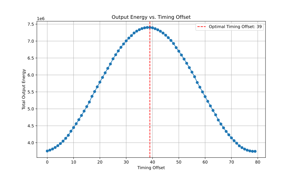
We will implement symbol synchronization using the technique discussed in class, which aims to find the timing offset that maximizes the so-called “output energy”, hence the name maximum output energy (MOE) symbol synchronization. Create a function that looks like this:
rx_symbols, offset = symbol_synch_moe(rx_signal,sps,upsample=8,plot=False)Here, rx_signal is the output of the matched filter (sampled at a rate of fs) and rx_symbols is the downsampled version of rx_signal (sampled at a rate of fs/sps).
Note that, since we have not performed frame synchronization, rx_symbols will contain the transmitted symbols along with noise before and after the desired transmitted symbol sequence; we will extract only the transmitted symbols during frame synchronization.
The upsample field sets the factor by which rx_signal is upsampled before performing MOE symbol synchronization.
In other words, with upsample=8, rx_signal will be increased in length by a factor of 8 by increasing its sampling rate via upsampling (inserting zeros and convolving with a low-pass filter); you will need to implement this upsampling function.
Use the plot flag to turn on and off plotting to help with debugging.
With that being said, it may be useful to create the following upsample_signal function.
upsampled_signal = upsample_signal(received_signal, upsample)On this upsampled version of rx_signal, you should search for the offset (a value between 0 and sps*upsample - 1) that maximizes the output energy when sampling the signal every $T$ seconds (i.e., every sps*upsample samples).
The output energy in this context is just the sum of the squared magnitude of the samples.
Plot the output energy as a function of offset. For reference, here’s what I see on my end.
Part III: Frame Synchronization
The next step is to extract the transmitted frame of symbols from rx_symbols.
To aid in this effort, we will add a training sequence to the beginning of our transmitted frame.
Begin by creating function that returns a Zadoff-Chu sequence of length N with root q.
zc = zadoff_chu_sequence(N,q)Then, use this to create a short-training field (STF) comprised of 16 repetitions of a length-19 Zadoff-Chu sequence. Use whatever root q you want.
After that, create a long-training field (LTF) comprised of two repetitions of a length-937 Zadoff-Chu sequence. Again, use whatever root q you want.
Prepend the STF and LTF to your frame, so that it looks like this. Place some zeros between the STF and LTF if you’d like.
┌─────┬─────────┬──────────┬──────────────┐
│ STF │   LTF   │  Pilots  │     Data     │
└─────┴─────────┴──────────┴──────────────┘
The STF should look like this, where SZC is the length-19 Zadoff-Chu sequence.
┌─────┬─────┬─────┬─────┐
│ SZC │ SZC │ ... │ SZC │
└─────┴─────┴─────┴─────┘
The LTF should look like this, where LZC is the length-937 Zadoff-Chu sequence.
┌─────────┬─────────┐
│   LZC   │   LZC   │
└─────────┴─────────┘
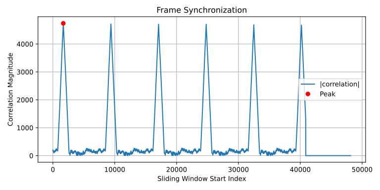
Use the LTF to perform frame synchronization by taking the inner product of each length-937 segment of the received symbols with the subsequent length-937 segment. The magnitude of this inner product should exhibit a peak where the LTF is. So you are aware, this is based on the method introduced by Schmidl-Cox.
Include in your lab report a plot of the magnitude of the inner product output during frame synchronization. For reference, here’s what I see on my end.
Part IV: Frequency Synchronization
In order to transmit and receive across two different SDRs, you will need to estimate and correct for CFO. To estimate CFO, we will use a two-staged approach where a coarse estimate of the CFO is found via the STF and a finer estimate is found via the LTF. It is important to make sure you apply coarse CFO correction to the received samples (including the LTF) before performing the finer CFO estimation via the LTF. The key advantage of this approach is that the STF can be used to estimate a wider range of CFO, but can be more susceptible to noise, whereas the LTF can be used to provide a more reliable estimate, but can only be used to estimate a narrower range of CFO.
Estimating the coarse CFO will be done via an extension of the Moose method discussed in class.
The key difference is that, instead of having only two copies, we have several copies of the short Zadoff-Chu sequence (SZC).
The received STF consists of 16 copies of the SZC.
Suppose you take copies 1 through 15 to form a vector x, and then take copies 2 through 16 to form a vector y.
If you find the phase difference between the i-th elements of x and y, then this should correspond to a phase that is proportional to the length of the SZC (which is 19).
This phase can be used to make a coarse estimate of the CFO.
Report the coarse CFO estimate and the maximum unambiguous CFO the STF can estimate.
Apply CFO correction to the received samples (including the LTF), and then repeat this process for the LTF. Since you only have two copies of the LZC, the approach you should use follows verbatim from the Moose method discussed in class. Report the fine CFO estimate and the maximum unambiguous CFO the LTF can estimate.
Part V: Channel Estimation, Channel Equalization, and Symbol Detection
Now, like done in Lab 3, use the transmitted pilots to perform channel estimation and then use this channel estimate to equalize your received signal by dividing it by this estimated complex gain.
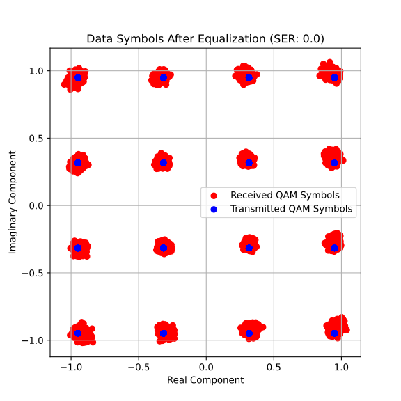
Plot the real and imaginary components of each received symbol on the complex plane after equalization, and then overlay the originally transmitted symbols. Report your symbol-error rate (SER) in the title of your plot. For reference, here’s what I see on my end.